


Time series forecasting lies at the heart of data-driven decision-making — from predicting stock prices and sales trends to anticipating energy consumption and weather patterns. By analyzing how data changes over time, we can uncover hidden structures, detect anomalies, and generate accurate predictions about the future.
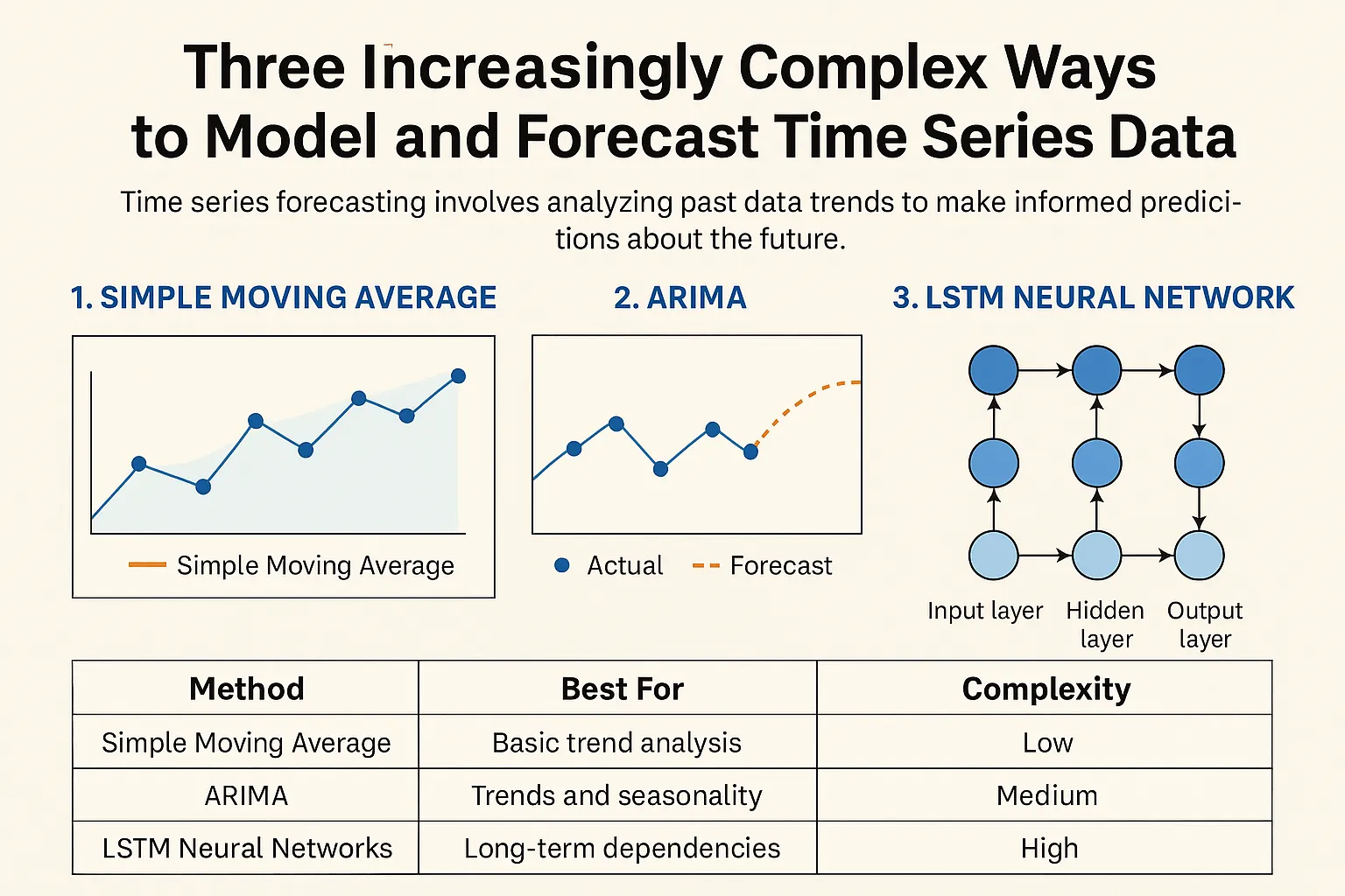
In this guide, we’ll explore three increasingly complex methods for modeling and forecasting time series data — starting with simple moving averages and advancing toward ARIMA models and deep learning LSTM networks. Each step introduces more sophistication, but also greater predictive power.
Why Model Time Series Data?
Time series analysis is about more than just predicting numbers — it’s about understanding the story behind them. Organizations use forecasting models to:
- Detect trends: Identify long-term patterns, cycles, and seasonality.
- Make predictions: Anticipate sales, demand, or performance metrics.
- Support decisions: Optimize inventory, allocate budgets, and plan production with greater confidence.
Let’s break down three major approaches — from simple to advanced — and see how each one builds on the last.
Method 1: Simple Moving Average (SMA)
The simplest form of time series forecasting, the Simple Moving Average smooths short-term fluctuations by averaging data over a fixed window. This makes it easier to observe underlying trends without being distracted by daily noise.
import pandas as pd
import matplotlib.pyplot as plt

# Sample data
data = {'Date': pd.date_range(start='1/1/2023', periods=10, freq='D'),
        'Sales': [10, 12, 13, 15, 18, 20, 22, 24, 26, 30]}
df = pd.DataFrame(data)
df.set_index('Date', inplace=True)

# Calculate a 3-day moving average
df['SMA_3'] = df['Sales'].rolling(window=3).mean()

df.plot(figsize=(10,5))
plt.title("Simple Moving Average Forecast")
plt.show()
The moving average is excellent for trend visualization — it filters out random fluctuations and highlights the general direction of the data. However, it’s less effective for forecasting sudden changes or seasonality.
Pros: Simple, fast, and ideal for exploratory analysis.
Cons: Lags behind real-time data and struggles with complex patterns.
Method 2: ARIMA — A Classic Statistical Approach
When you need more accuracy, the Autoregressive Integrated Moving Average (ARIMA) model steps in. ARIMA captures the dependencies between past and present data points and can model both trends and seasonality.
It’s composed of three parameters: (p, d, q) — where p is the autoregressive term, d is the differencing order (to make data stationary), and q is the moving average component.
from pmdarima import auto_arima
from statsmodels.tsa.arima.model import ARIMA
import matplotlib.pyplot as plt

# Automatically find best ARIMA parameters
model = auto_arima(df['Sales'], seasonal=False, trace=True)
order = model.order

# Fit model
arima_model = ARIMA(df['Sales'], order=order)
fit = arima_model.fit()

# Forecast 5 future points
forecast = fit.forecast(steps=5)

# Plot results
plt.figure(figsize=(10,5))
plt.plot(df.index, df['Sales'], label="Actual Sales")
plt.plot(pd.date_range(df.index[-1], periods=6, freq='D')[1:], forecast,
         label="Forecast", linestyle='dashed')
plt.legend()
plt.title("ARIMA Forecast")
plt.show()
ARIMA models are a workhorse for short- to medium-term forecasting, particularly when historical data shows consistent patterns or seasonality.
Pros: Captures trends, seasonality, and autocorrelation effectively.
Cons: Requires data stationarity and careful parameter tuning.
Method 3: Long Short-Term Memory (LSTM) Networks
When linear models reach their limit, deep learning takes over. Long Short-Term Memory (LSTM) networks are a type of recurrent neural network (RNN) designed to handle sequential data and remember information across long time horizons — making them ideal for complex, non-linear patterns.
import numpy as np
from sklearn.preprocessing import MinMaxScaler
import tensorflow as tf

# Scale data
scaler = MinMaxScaler()
df['Sales_scaled'] = scaler.fit_transform(df[['Sales']])

# Prepare sequences for training
def create_sequences(data, seq_length=5):
    X, y = [], []
    for i in range(len(data) - seq_length):
        X.append(data[i:i+seq_length])
        y.append(data[i+seq_length])
    return np.array(X), np.array(y)

X, y = create_sequences(df['Sales_scaled'].values, seq_length=5)
X = np.expand_dims(X, axis=2)

# Define LSTM model
model = tf.keras.Sequential([
    tf.keras.layers.LSTM(64, return_sequences=True, input_shape=(5, 1)),
    tf.keras.layers.LSTM(32),
    tf.keras.layers.Dense(1)
])
model.compile(optimizer='adam', loss='mse')
model.fit(X, y, epochs=50, batch_size=1, verbose=0)
LSTMs excel at identifying long-term dependencies — for example, how sales trends depend not just on last week’s data but on patterns from months ago. They’re used in fields such as stock prediction, energy consumption forecasting, and weather modeling.
Pros: Excellent for nonlinear, long-term dependencies.
Cons: Requires more data and computational resources; harder to interpret.
Comparing the Three Methods
Each approach offers unique strengths depending on the use case, data quality, and complexity requirements.
| Method | Best For | Complexity | Accuracy |
|---|---|---|---|
| Simple Moving Average | Quick trend smoothing | Low | Low–Moderate |
| ARIMA | Structured, stationary time series | Medium | High |
| LSTM Neural Networks | Complex, nonlinear time series with long dependencies | High | Very High |
Choosing the Right Forecasting Technique
Start with simplicity. Moving averages are great for quick insights and small datasets. ARIMA comes next, offering a balance between statistical rigor and interpretability. When your data grows more complex or nonlinear — such as in sensor readings, speech, or energy demand — LSTM networks provide the most flexibility and power.
It’s often beneficial to combine techniques. For example, you might use ARIMA to capture seasonal patterns and feed residual errors into an LSTM model for final predictions — a hybrid approach that blends the best of both worlds.
FAQs
What is the difference between ARIMA and LSTM?
ARIMA relies on linear relationships and is interpretable, while LSTM learns complex nonlinear dependencies. ARIMA is faster to train, but LSTM is often more accurate for large, intricate datasets.
How do I know if my data is stationary?
You can check stationarity using visual inspection (flat mean/variance) or statistical tests like the Augmented Dickey-Fuller (ADF) test.
Do I always need deep learning for time series?
No — simple models often perform just as well. Deep learning adds value mainly when your data has multiple variables, nonlinear relationships, or long-term dependencies.
What tools are best for time series forecasting?
For Python: statsmodels, pmdarima, prophet, and tensorflow are top libraries, each suited to different complexity levels.
Can I combine multiple forecasting models?
Yes. Ensemble and hybrid models often outperform single models, especially when combining statistical and machine learning methods.
Conclusion
Time series forecasting is both an art and a science. Whether you’re smoothing data with a moving average, fine-tuning ARIMA parameters, or training deep learning models, the key lies in experimentation and understanding your data’s behavior. Start simple, build confidence, and gradually move toward more sophisticated models as your needs evolve.
The more you explore your data’s patterns, the more accurate — and actionable — your forecasts will become.